Quick Links
- Introduction
- The need for hybrid search
- The anatomy of hybrid search in OpenSearch
- Some limitations of hybrid search
- Let’s conclude
Introduction
This article is the third in a series of five that dives into the intricacies of vector search (aka semantic search) and how it is implemented in OpenSearch and Elasticsearch.
This first part: A Quick Introduction to Vector Search, was focused on providing a general introduction to the basics of embeddings (aka vectors) and how vector search works under the hood. The content of that part was more theoretical and not oriented specifically on OpenSearch, meaning that it was also valid for Elasticsearch as they are both based on the same underlying vector search engine: Apache Lucene.
Armed with all the vector search knowledge learned in the first article, the second article: How to Set Up Vector Search in OpenSearch, guided you through the meanders of setting up vector search in OpenSearch using either the k-NN plugin or the new Neural Search plugin that was recently made generally available in version 2.9.
In this third part, we are going to leverage what we’ve learned in the first two parts and build upon that knowledge by delving into how to craft powerful hybrid search queries in the newly released OpenSearch 2.10.
The fourth part: How to Set Up Vector Search in Elasticsearch and the fifth part: Elasticsearch Hybrid Search of this series will be similar to the second and third ones but focused on Elasticsearch.
The need for hybrid search
Before diving into the realm of hybrid search, let’s do a quick refresh of what we learned in the first article of this series regarding how lexical and semantic search differ and how they can complement each other.
To sum it up very briefly, lexical search is great when you have control over your structured data and your users are more or less clear on what they are searching for. Semantic search, however, provides great support when you need to make unstructured data searchable and your users don’t really know exactly what they are searching for. It would be fantastic if there was a way to combine both together in order to squeeze as much substance out of each one as possible. Enter hybrid search!
In a way, we can see hybrid search as some sort of “sum” of lexical search and semantic search. However, when done right, hybrid search can be much better than just the sum of those parts, yielding far better results than either lexical or semantic search would do on their own.
Running a hybrid search query usually boils down to sending a mix of at least one lexical search query and one semantic search query and then merging the results of both. The lexical search results are scored by a similarity algorithm, such as BM25 or TF-IDF, whose score scale is usually unbounded as the max score depends on the number and frequency of terms stored in the inverted index. In contrast, semantic search results can be scored within a closed interval, depending on the similarity function that is being used (e.g., [0; 2] for cosine similarity).
In order to merge the lexical and semantic search results of a hybrid search query, both result sets need to be fused in a way that maintains the relative relevance of the retrieved documents, which is a complex problem to solve. Luckily, there are several existing methods that can be utilized; two very common ones are Convex Combination (CC) and Reciprocal Rank Fusion (RRF).
Basically, Convex Combination, also called Linear Combination, seeks to combine the normalized score of lexical search results and semantic search results with a weight (where 0 1), such that:

CC can be seen as a weighted average of the lexical and semantic scores, where all weights are expressed as percentages, i.e., they add up to 100%.
RRF, however, doesn’t require any score calibration or normalization and simply scores the documents according to their rank in the result set, using the following formula, where k is an arbitrary constant meant to adjust the importance of lowly ranked documents:

Both CC and RRF have their pros and cons as highlighted in Table 1, below:
Table 1: Pros and cons of CC and RRF
| Convex Combination | Reciprocal Rank Fusion | |
|---|---|---|
| Pros | - Good calibration of weights makes CC more effective than RRF | - Doesn’t require any calibration - Fully unsupervised - No need to know min/max scores |
| Cons | - Requires a good calibration of the weights - Optimal weights are specific to each data set | - Not trivial to tune the value of k - Ranking quality can be affected by increasing result set size |
It is worth noting that not everyone agrees on these pros and cons depending on the assumptions being made and the data sets on which they have been tested. A good summary would be that RRF yields slightly less accurate scores than CC but has the big advantage of being “plug & play” and can be used without having to fine-tune the weights with a labeled set of queries.
Up until version 2.10, hybrid search was just a dream in OpenSearch, and the only way to achieve it was to send queries separately and perform all the merging logic in the client application as demonstrated in this excellent blog. As of 2.10, hybrid search in OpenSearch is finally a reality, exactly one year after Elasticsearch released the feature in 8.4. Let’s now see how that was made possible.
The anatomy of hybrid search in OpenSearch
In contrast to Elasticsearch, which went the RRF way as of version 8.8, the OpenSearch community has decided to implement hybrid search with the CC approach by normalizing the relevance scores of both result sets to the same scale so they can easily be further combined. If you are interested in reading more about score normalization and combination techniques, you can check out this blog written by top-notch AWS engineers.
Introducing the new hybrid query
Now, let’s get down to the real meat! The latest 2.10 release of OpenSearch (September 13th, 2023) provides a new query called `hybrid`, which allows users to specify an array of queries composed of at most five lexical (i.e., `term`, `match`, `match_phrase`, etc.) and semantic (e.g., `neural`, `knn`) search queries. The code block below shows what this new `hybrid` query looks like:
{
  "query": {
    "hybrid": {
      "queries": [
        {
          "match": {
            "field": {
              "query": "lorem ipsum"
            }
          }
        },
        {
          "neural": {
            "field": {
              "query_text": "dolor sit amet",
              "model_id": "my-model-id",
              "k": 3
            }
          }
        }
      ]
    }
  }
}
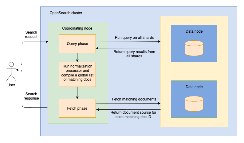
When such a query is sent by the client, the coordinator node sitting on the front lines will first analyze all the queries composing the `hybrid` query (i.e., `match` and `neural` in the example above) and forward each of them to all the shards of the index(es) being queried. Each shard will then run the queries locally and return the matching doc IDs and their local relevance scores to the coordinating node. A document can be returned if it matches at least one of the specified queries. This part is called the query phase.
When the query phase is over, i.e., when all the shards have returned their local results, the coordinator node needs to perform the fetch phase, which consists of a second round-trip to fetch the actual content of the top matching documents. However, before it can proceed, it needs to determine the top matching documents by normalizing and combining the shard-local relevance scores into a global result list. The way this is done in OpenSearch is by leveraging search pipelines, which have been available since version 2.8. Figure 1, below, shows the overall process that we have just described:
Figure 1: Score normalization running between the query and fetch phases

Introducing the new search pipeline normalization processor
Similar to ingest pipelines running at indexing time, search pipelines kick in at search time and allow users to run a variety of processors that can operate on both the search query and search results as well as between the query and fetch phases. There are three types of search processors: request processors (running before the query phase), phase results processors (running between the query and fetch phases), and response processors (running after the fetch phase).
The type of processor that we are going to use in order to perform this score normalization is a phase results processor called the `normalization_processor`. In order to leverage this new processor type, we need to create a search pipeline called `hybrid-search-pipeline`, as shown below:
PUT /_search/pipeline/hybrid-search-pipeline
{
  "description": "Score normalization processor for hybrid search",
  "phase_results_processors": [
    {
      "normalization-processor": {
        "normalization": {
          "technique": "min_max"
        },
        "combination": {
          "technique": "arithmetic_mean",
          "weights" : [0.4, 0.6]
        }
      }
    }
  ]
}
We can see that the `normalization_processor` takes a few optional configuration parameters that are described in Table 2, below:
Table 2: Configuration parameters for the normalization processor
| Parameter name | Type | Description |
|---|---|---|
| normalization.technique | String | The name of the score normalization technique to use. The valid values are `min_max` (default) and `l2`. More details about these normalization techniques can be found here. |
| combination.technique | String | The name of the score combination technique to use. The valid values are `arithmetic_mean` (default), `geometric_mean`, and `harmonic_mean`. More details about these combination techniques can be found here. |
| combination.parameters.weights | Float[] | The weights (between 0.0 and 1.0) to use for each query. The array must have the same number of weights as the number of hybrid queries, and their sum must equal 1.0. |
Let’s now see how this works on a concrete example.
An illustrative example
Remember the `neural` search query that we introduced toward the end of the second article of this series? Now, we are going to use that same query in conjunction with a lexical `match` query to perform a hybrid search using the search pipeline we have just defined, which will normalize and combine the relevance scores of the lexical and semantic search results:
POST main-index/_search?search_pipeline=hybrid-search-pipeline
{
  "size": 3,
  "_source": [
    "text-field"
  ],
  "query": {
    "hybrid": {
      "queries": [
        {
          "match": {
            "text-field": {
              "query": "fox"
            }
          }
        },
        {
          "neural": {
            "vector-field": {
              "query_text": "Who jumps over a dog?",
              "model_id": "O7IV2YkBFKz6Xoem-EFU",
              "k": 3
            }
          }
        }
      ]
    }
  }
}
Let’s now take it all apart and describe the steps that are going to be executed in order to carry out this hybrid search query:
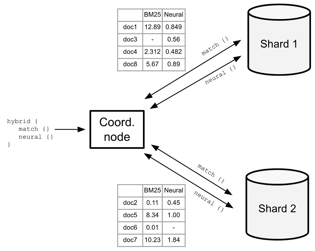
1. The coordinator node will send the `match` and `neural` search queries to all the shards of the `main-index` index (see Figure 2, below).
2. Each shard will return the doc IDs and the raw BM25 scores of the lexical match results (column B in Table 3) as well as the doc IDs and the raw scores of the semantic match results (column E in Table 3) as shown in Figure 2, below:
Figure 2: Returning local results from each shard

3. The coordinator node gathers all shard-local query phase results and runs them through the `hybrid-search-pipeline` as can be seen in Table 3, below, which summarizes what the score normalization and combination process looks like on a fictional result set:
- The `normalization-processor` phase result processor will first normalize all the lexical and neural search scores in the [0.0; 1.0] range using the min-max normalization formula shown below (columns C and F):

- And then combine them with the following arithmetic mean formula (columns D, G, and H) using the weights specified in the search pipeline:

Table 3: Score normalization and combination process
| A | B | C | D | E | F | G | H | I |
|---|---|---|---|---|---|---|---|---|
| BM25 | BM25 normalized | BM25 weighted | Neural | Neural normalized | Neural weighted | Combined score | Final rank | |
| doc1 | 12.890 | 1.000 | 0.400 | 1.63 | 0.849 | 0.509 | 0.455 | 2nd |
| doc2 | 0.110 | 0.008 | 0.003 | 0.45 | 0.000 | 0.000 | 0.002 | |
| doc3 | 0.000 | 0.000 | 0.56 | 0.079 | 0.047 | 0.024 | ||
| doc4 | 2.312 | 0.179 | 0.072 | 1.12 | 0.482 | 0.289 | 0.180 | |
| doc5 | 8.340 | 0.647 | 0.259 | 1.00 | 0.396 | 0.237 | 0.248 | 3rd |
| doc6 | 0.010 | 0.000 | 0.000 | 0.000 | 0.000 | 0.000 | ||
| doc7 | 10.230 | 0.793 | 0.317 | 1.84 | 1.000 | 0.600 | 0.459 | 1st |
| doc8 | 5.670 | 0.439 | 0.176 | 0.89 | 0.317 | 0.190 | 0.183 |
4. Finally, the coordinator node takes the top three (k = 3) documents with the highest global scores, i.e., doc7, doc1, and doc5 (column I), and returns them to the client.
A more concrete example
Remember the “I’m not right” example from the first article? Let’s see how this new `hybrid` search feature can help us retrieve more accurate results.
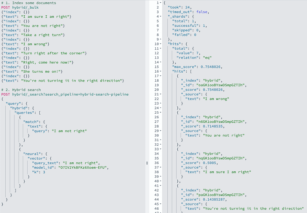
Figure 3, below, shows that searching for “I am not right” using the `hybrid` search query composed of a lexical `match` query and semantic `neural` query now returns a much more accurate result, namely “I am wrong”, which is exactly what we were expecting. Also note that we are leveraging the `hybrid-search-pipeline` we created earlier, which ponderates the lexical and semantic search queries with 0.4 and 0.6 weights.
Figure 3: Hybrid search returning even more accurate results

A final comparison
In the previous article, we saw how k-NN and neural searches can improve the quality of search results. In this one, we went one step further and showed how hybrid search queries combining lexical and semantic search queries can further increase the quality of the returned results. Table 4, below, gives a quick recapitulation of the search results returned by each query type:
Table 4: Recapitulation of all types of semantic search queries seen so far
| Query type | Pure lexical | Pure vector | Hybrid |
|---|---|---|---|
| query": "I am not right" | match": {} | neural": {} / "knn": {} | "hybrid": {"match"+"neural"} |
| Results: | |||
| 1st hit | "I am sure I am right" | "You are not right" | "I am wrong" |
| 2nd hit | "I am wrong" | "I am wrong" | "You are not right" |
| 3rd hit | "You are not right" | "I am sure I am right" | "I am sure I am right" |
As we can see, the only query that captures the real meaning of the user input is the hybrid one, which returns “I am wrong” as the first result. Admittedly, this is a very simplified example, and depending on your dataset your mileage may vary, but it still illustrates the value of hybrid search. You will probably need to experiment a little in order to figure out the optimal query weights as well as the best ways to query your dataset.
Some limitations of hybrid search
When new features are released, they usually come with some limitations as concessions often have to be made to meet market windows and release deadlines. The new `hybrid` search query is no exception to the rule, so let’s quickly look at some of the current limitations:
- Filtering is not yet available for hybrid queries the same way they are available for k-NN queries. However, as pointed out in this issue and even if that can be inconvenient to specify the same filter multiple times, it is still possible to provide them inside each of the sub-queries in `bool/filter` queries.
- Pagination is not yet supported (see this issue)
- The Explain API does not yet support explaining hybrid queries, this will be addressed in a second phase
- All subqueries are currently being executed sequentially, work is in progress to make them execute in parallel (see this issue)
Also, the requirement of having to specify weights within the search pipeline could be seen as a limitation because it means that each hybrid search query might require a dedicated search pipeline depending on how many subqueries it contains and which index (i.e., data set) it is executed against.
Let’s conclude
In this article, we have introduced the new `hybrid` search query and the new `normalization-processor` search pipeline processor released in OpenSearch 2.10, which together enable hybrid search queries.
We first did a quick recap of the many advantages of being able to fuse lexical and semantic search results in order to increase accuracy. Along the way, we reviewed two different methods of fusing lexical and semantic search results, namely Convex Combination (CC) and Reciprocal Rank Fusion (RRF) and looked at their respective pros and cons.
Then, using an illustrative example, we showed how OpenSearch has implemented the whole hybrid search process using Convex Combination, and we concluded by listing a few limitations of the current hybrid search implementation.
If you like what you’re reading, make sure to check out the other parts of this series:
- Part 1: A Quick Introduction to Vector Search
- Part 2: How to Set Up Vector Search in OpenSearch
- Part 4: How to Set Up Vector Search in Elasticsearch
- Part 5: Hybrid Search Using Elasticsearch


